Data science, two words which even the initiated have trouble with explaining to the layperson. There's an old saying that if you can't explain it to your grandmother, you probably do not understand it well enough. That stands very true, especially today in 2016, given the complexities that more often than not plague most intellectual endeavors. Personally my favorite go-to line when I'm on the receiving end is - Please explain to me as you might to a child, or a golden retriever.
So yes, jokes aside where do we begin. The example that works best for me is, you know how Amazon will show and recommend you stuff like the things you have browsed and bought? And you end up buying things in addition to what you browsed for? That is data science/machine learning going down. In the flesh. Simple.
Recommender engines are machine learning examples which everyone understands because they are all around us, like Netflix, Amazon, Youtube etc. It's fun to observe them even, say when Spotify recommends you this cool new artist because it saw you listening to The Black Keys. We see it communicating and interacting with us, although that might not always be the case. An example of a recommendation engine which might be a little furtive is Gmail deciding whether an incoming mail is spam or not.
A music recommender is even more exciting because it is tangible. Even though music taste is so personal and inexplicable, modern recommenders do a good job of suggesting tracks we did not know we would like.
The Data Set
The dataset for this recommender is published by Audioscrobbler, the music recommendation system for last.fm. Last.fm was one of the first modern Internet streaming radio sites which gained rapid popularity in the mid-2000s. Audioscrobbler provided the capabilties for scrobbling or recording user's plays of songs. Last.fm relied on this information to make recommendations to users about artists and songs they might like.
The dataset is interesting, because when last.fm was blowing up most recommendation engines relied on rating-like data. They ingested inputs like - Guneet gave Metallica 4/5. This is where Audioscrobbler got interesting because it simply recorded plays. The familiar - "Guneet played Walk by Pantera". We should be careful here and realize that ratings and plays carry different meanings. Just because I played a track does not neccesarrily mean I actually liked it. A lot of times you would play anything and just be doing your daily chores. The catch is that a listener is much more likely to play music than to give an actual rating. Therefore scrobbled data is MUCH larger and covers more users and artists. That is a lot more information than a rating data set even though each individual point would carry less of the same.
A snapshot of such a scrobbled music data is what we are looking at. It was published by last.fm in 2005 and can be found here. The main data is in the user_artist_data.txt file.
Essentially, what we are looking at is -
- 141,000 unique users
- 1.6 million unique artists
- 24.2 million users
What we also have are the artist_data.txt and artist_alias.txt files. The former gives the name of artist by ID, the latter maps artist IDs that are known misspellings or variants to the canonical artist ID. Say, "The Corrs", "Corrs", "the corrs" may appear as distinct artist IDs in the data set, even though they are the same.
Since we are looking at some big numbers here, I thought to run the analysis on an AWS cluster using Apache Hadoop and Spark. A LOT of this was also experimented and worked on my local Macbook running Spark on VMware.
Motivation
This has also been my first foray in getting comfortable with Scala, hence some screenshots have been taken over a period of time and improved on. It's been a great learning experience and I owe a lot to the powerful Vincent Singhania and Scooby. A big thank you to Sandy Ryza and Sean Owen (this article learns from his work and techniques in Advanced Analytics with Spark). Apache Spark offers a Python wrapper, PySpark, but my motivation to use Scala was manyfold, namely -
- I wanted to learn a new language!
- The Spark framework is written in Scala. This offers a number of advantages, such as reduced performance overhead and access to all of spark's access libraries.
- Understand what's going down under the hood, ala "think in Spark".
Last but not the least, this has also been a selfish venture of sorts. To make things clear, I was an avid last.fm user during 2004-2008. My own personal scrobbled data is in there!
The Recommender Algorithm
The data consists entirely of interactions between users and artists songs, but has no user and artist information other than their names. We need an algorithm that would learn without access to either user or artist attributes. Collaborative filtering algorithms meet this criteria. Collaborative filtering would decide that two users may both like the same song because they play many other same songs. Deciding that two users might have similar music tastes because they are of the same age is not example that would come under this umbrella.
We use an alternating least squares (ALS) recommender here. It is a type of matrix factorization model. We treat the user and product data as if it were a large matrix A, where an entry at row i and column j exists if user i has played artist j. A is sparse: owing to only a few off all possible user-artist combinations appearing in the data, most entries are 0. The matrix A can be factored as the matrix product of two smaller matrices X and Y. Both of them have many rows because A has many rows and columns, but just a few columns k. The columns correspond to the latent factors that are being used to explain the interaction data.
ALS computes X and Y. We will not going into detail the workings of the algorithm here. The approach was popularized by papers like Collaborative Filtering for Implicit Feedback Datasets and Large scale Parallel Collaborative Filtering for the Netflix Prize. It rose to prominence during the time of the Netflix Prize. On 21 September 2009, Bellgor's Pragmatic Chaos Team bested Netflix's own alrogithmic for predicting ratings by ~10% and won the prize worth US $1,00,000.
ALS takes advantage of sparsity of the input data and relies on simple and optimized linear algebra. It's data parallel nature makes it very fast at a large scale. And last but not the least, ALS is the only recommender algorithm currently implemented in the Spark machine learning library, haha.
Data Preparation
All three data files are being stored in HDFS. While starting the spark-shell remember to specify --driver-memory 6g to have sufficient memory to complete these computations. I'm assuming that you are kind of familiar with the Apache Spark environment and know your way around.
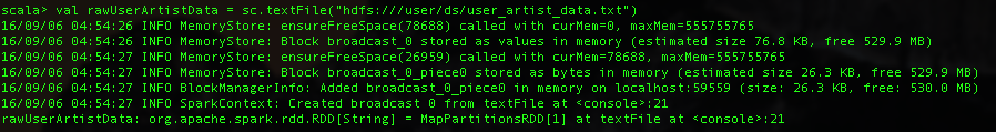
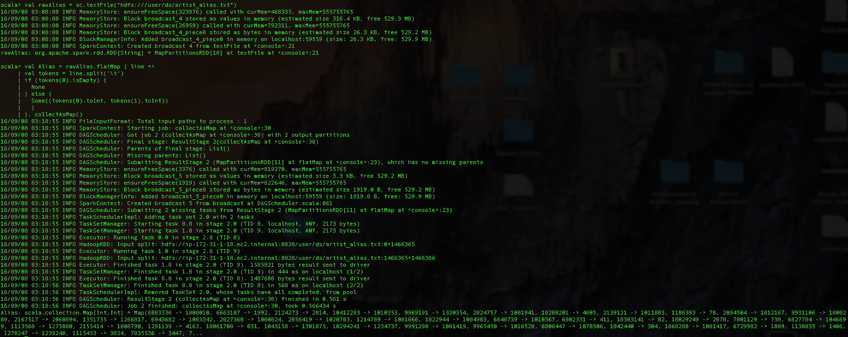
One limitation of Spark MLib's ALS implementation is that it requires numeric nonnegative 32-bit integers IDs for users and items. This means that IDs larger than about Integer.MAX_VALUE or 2147483647 cannot be used. Let's load up the data and see if this is meet. We access the file as an RDD of Strings with SparkContext's textFile method.

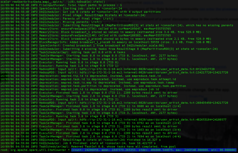
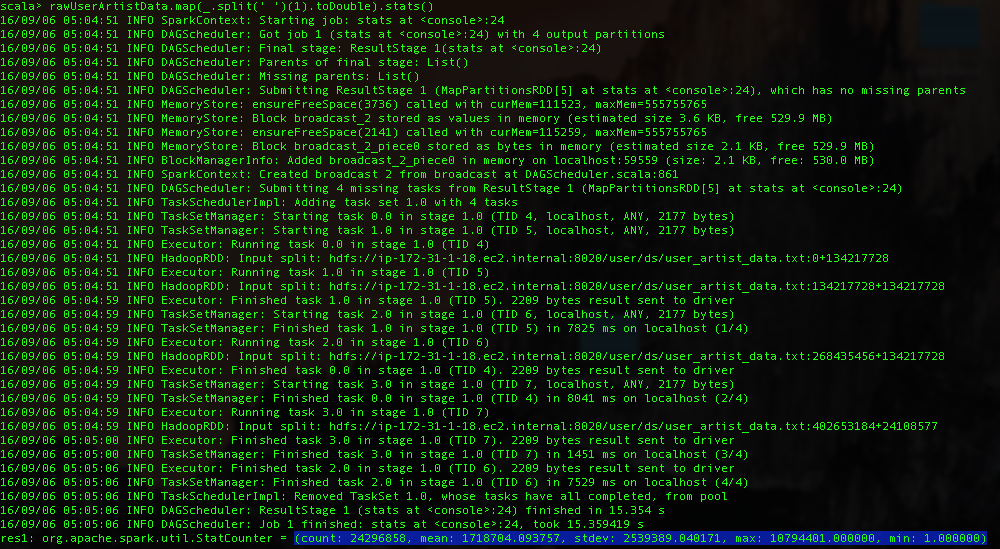
Each line of the file contains a user ID, an artist ID and a play count, separated by space. We compute statistics on the user and artist IDs using the stats() method.
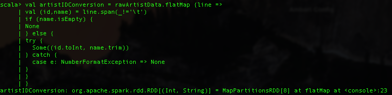
Next lets convert the artist names corresponding to the numeric IDs. artist_data.txt contains the artist ID and name separated by a tab.

The artist_alias.txt file maps artist IDs that might be misspelled to the canonical artist name. It consists of two IDs per line, separated by a tab. We use it to map incorrect artist IDs to correct ones.
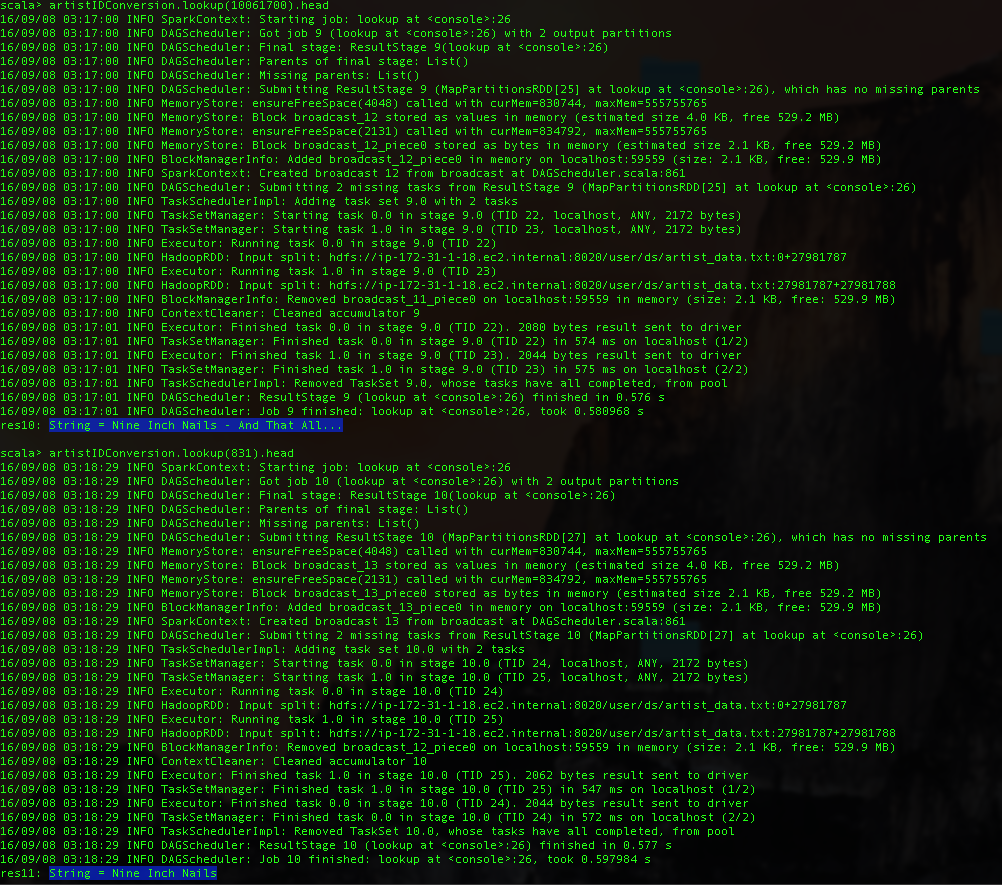
The entry 10061700 maps to entry 831. We can look these up from the RDD containg artist names, to see that the particular ID corresponds to the 90s industrial metal powerhouse Nine Inch Nails. We fixed "Nine Inch Nails - And That All..." to the correct artist name "Nine Inch Nails".
Model
Although the dataset is almost in the right form for use with Spark's ALS implementation, we require two transformations. First we should convert all artist IDs to canonical IDs using our aliases data set incase of existence of multiple canonical IDs. Second, the data should be converted into Rating objects, which is the implementation's abstraction for user-product-value data. Product here refers to artists.
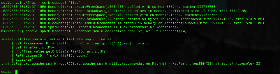
We used a broadcast variable here, bAlias, for our artist alias. Broadcast variables come in handy when you have a large number of tasks that need to handle the same data structure. It enables caching of data across multiple stages and jobs, saving significant network traffic and memory.
The ALS algorithm being iterative, will need to access this data numerous times which is why we use cache() to tell Spark that this particular RDD should be stored temporarily after being computed and keep it in memory in the cluster. If we don't do this the RDD could be computed repeatedly each time it is accessed from the original data.
Alright, so FINALLY, we can build the model!

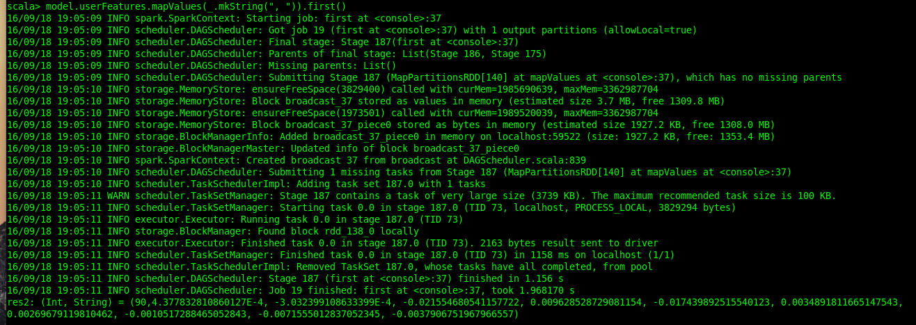
This operation will take some time to construct our matrix factorization model, simply because the model is huge. We are looking at a feature vector of 10 values for each user and product, and there are around a million and a half of them :) These large user-feature and product-feature matrices in the model are RDDs of their own. You would notice a bunch of arguments in the trainImplicit() call above, and I'll go into them shortly. We can see some of these feature vectors. Each feature vector is an array of 10 numbers and we print it using mkString(). It translates the arrays into redable form.
Alright, who's ready to see some artist recommendations! Let's take a user, extract the artists this user has listened to and print 'em.
Let's pick user '2012130' ...

And collect his unique artists...

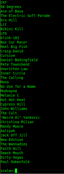
And just grab the artist names out of the selection. Print 'em...
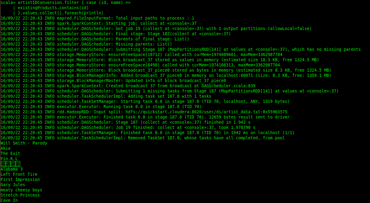
All of 'em...
Let's make some recommendations for our user - 2012130. 5 recommendations seems like a good number. We will extract out artist IDs and look up the artist names on the basis of the estimate that user will or won't interact with the artist. This estimate is obtained from the ALS algorithm as a rating value between 0 and 1. A higher value wherein translates to a better recommendation. It is not a probability though.

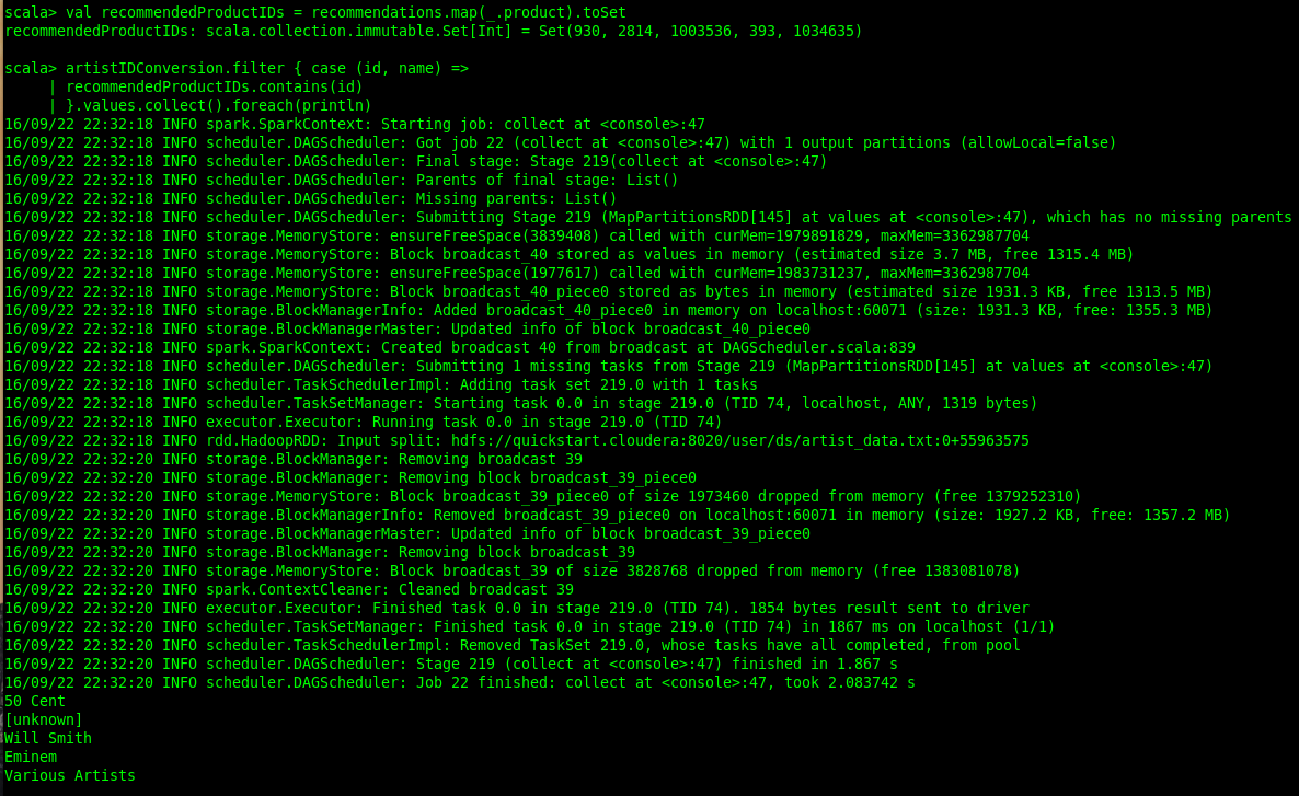
We obtain our 5 recommendations as shown above. It's interesting to note that an 'unknown' artist sneaked into our recommendation. I'll be addressing this shortly when we evaluate the quality of our recommendations. Other than that its a hip-hop heavy recommendation list with 50 Cent, Eminem and Will Smith.
Recommender Quality
Now recommending music is a tricky business. It's pretty subjective and its hard for anyone but the user to evaluate how good the recommendations are. Fair assumptions would assume that the user would tend to play songs from artist who he/she finds appealing and will not play artists who are not. And the plays (scrobbling) would only give us a partial picture of likes and dislikes.
The recommender recognises 'good' artists as the artists the user has listened to. What we do not want is the algorithm returning the previously listened to artists to the user and score perfectly. For this scenario we build the ROC (Receiver Operator Characteristic) curve and calculate the area under the curve (AUC). We test our model using hold-out validation.
I will not go into the details of the ROC curve and the validation technique, but to summarize it briefly we set aside some of the play data and hide it from the model building process. This held out data is collection of good recommendations which the model will not see. The recommender ranks all items in the model and it's score is calculated by comparing theh ranks of all items and ranks of the all held-out artists. 1 is a perfect score, 0 is the worst and 0.5 would be score achieved from guessing randomly.
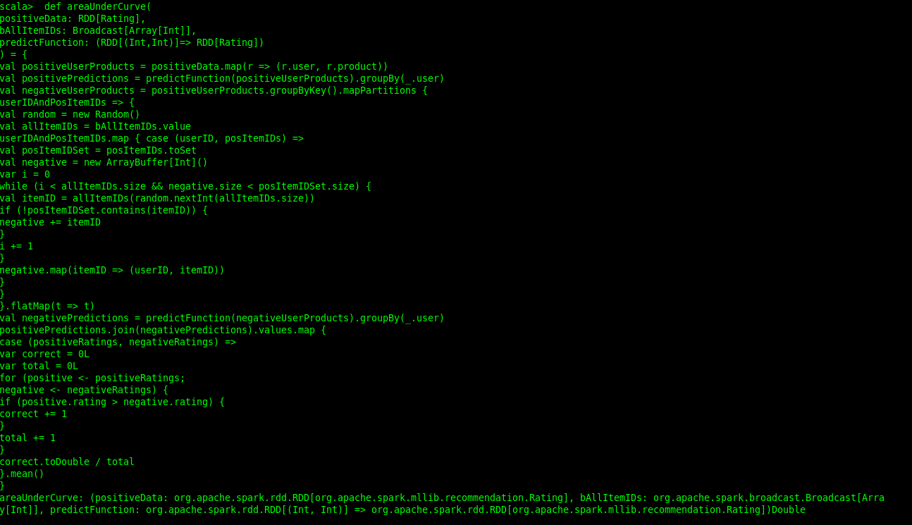
We divide our dataset into two parts, training (90%) and cross-validation (10%). The model is trained on the training data set only and evaluated against the cross-validation data set. The implementation code for calculating the AUC is complex whereby we are actually computing AUC per user and then a mean value is obtained across all users. AUC may be viewed as a probability that a randomn positive item sores higher than a negative one. We calculate the proportion of all positive-negative pairs that are correctly ranked. The held out data is taken as positive and we create a set of negative products for each user.
Let's build up our area under the curve function...
And divide the dataset..

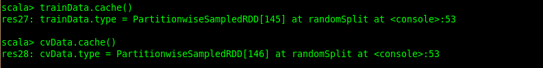
Cache them.
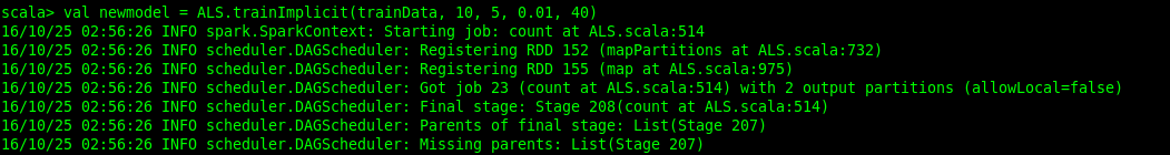
And create a new model with the training set...
Let's finally see how good our recommendations are then...

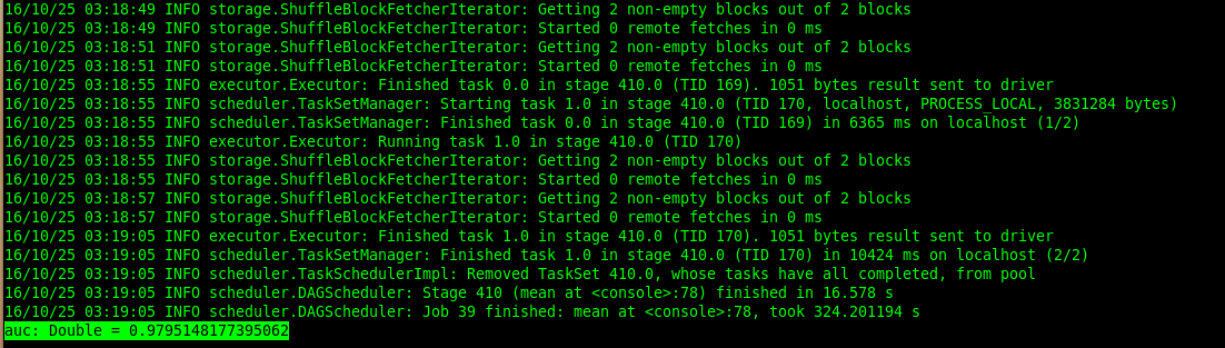
We got an AUC value of 0.979. It's definitely higher than 0.5 which would amount to recommending randomnly and pretty close to 1.0 which is the max score.
There were a couple of arguments passed to ALS.trainImplicit() aside from the training data. Let's discuss them.
-
Rank - 10
This corresponds to latent factors in the model, the number of columns in the product-feature and user-feature matrices (k). -
Iterations - 5
This corresponds to the number of iterations that the factorization runs. It can be thought of as a constraint trade off between time and better factorization. -
Lambda - 0.01
Lambda represents an overfitting parameter. Overfitting can be avoided by higher values but are subject to affecting factorization accuracy. -
Alpha - 40
This is responsible for the relative weight of unobserved vs observed user-product interactions in factorization. A higher alpha tends to make the model more confident about missing data equating to no preference for the particular user item pair. Think of it as the model would focus far more on what the user listened to than what he/she did not listen to. 40 was a value found to be optimum by experimenting in this case and is also recommended as a default by ALS documentation.
Choosing ideal values for these parameters for the desired scenario is a common task in machine learning. One of the common ways to deal with this is simply trial and error and going with the hyperparameter set that produces the best results.
Interestingly we observed an 'unknown' artist as one of the recommendations. Obviously, 'unknown' is not an artist, and we should discard all 'unknown' artist occurences in the dataset to fine tune our model. Our recommendations are as good as the data we have, which is why the bulk of the time of most data science endeavors is spent in cleaning the dataset.
Next Steps
We can spend some more time fine tuning our model by experimenting with different hyperparameters and removing anomalies in the data such as the 'unknown' artist. We can use the above scenario to also recommend users to artists. It can help us answer some really cool questions like what group of users would be the most interested in ,say, the new DMX album. This can be done by reading the artist as a user to recommend to, and the user as an artist.
As of now we can recommend to one user at a time using Spark Mllib's ALS implementation. However, we can rapidly compute recommendations for a group of users as part of multiple jobs, each of which take a few seconds to run. For faster lookups at runtime these recommendations can be written to an external NoSQL data store like HBase. Recommendations can be precomputed for all possible users and stored. But let's say if only a portion of the total users visit the site everyday, precomputing recommendations for all users (~millions) is a lot of wasted effort. Real-time recommendation systems are a way around this and utilize other modelling technique which are faster to implement.
Comments
comments powered by Disqus